Lossless Image Compression Algorithms Comparison
This post presents an analysis of different lossless image compression techniques applied to four images: three real-world images (baboon, house, and lake) and a randomly generated image. All images are PGM files, i.e. grayscaled images with 256 different gray levels, resulting in a bit-per-pixel (bpp) value of 8 before compression.
To compress an image, it would be sufficient to identify an error model through which the image deviates from a predicted image generated by predicting each pixel from the previous ones. This approach is likely to reduce the number of bits used, especially in images where pixels are highly dependent on each other.
Our example images are:


Calculation process
For the data processing process, MATLAB was used, specifically I relied on the following functions defined by me:
function [predictor] = advanced_predictor_calc(image)
    [rows, cols] = size(image);

    predictor = zeros(rows, cols);

    for n = 1:rows
        for m = 1:cols
            if n == 1 && m == 1
                predictor(n,m) = 128; % image(n,m) - 128;
            elseif n == 1
                predictor(n,m) = image(n,m-1);
            elseif m == 1
                predictor(n,m) = image(n-1,m);
            elseif m == cols
                predictor(n,m) = median([image(n-1,m), image(n,m-1), image(n-1,m-1)]);
            else
                predictor(n,m) = median([image(n-1,m), image(n,m-1), image(n-1,m+1)]);
            end
        end
    end
end

function [predictor] = simple_predictor_calc(image)
    [rows, cols] = size(image);

    predictor = zeros(rows, cols);

    for n = 1:rows
        for m = 1:cols
            if m == 1 && n == 1
                predictor(n,m) = 128;
            elseif  m == 1
                predictor(n,m) = image(n-1, cols);
            else
                predictor(n,m) = image(n, m-1);
            end
        end
    end
end

function [prediction_error] = advanced_prediction_error_calc(image)

    predictor = advanced_predictor_calc(image);
    prediction_error = int16(image)-int16(predictor);

end

function [prediction_error] = simple_prediction_error_calc(image)

    predictor = simple_predictor_calc(image);
    prediction_error = int16(image)-int16(predictor);

end

function [entropy] = entropy_calc(distribution)
    [counts, ~] = histcounts(distribution, unique(distribution));
    probabilities = counts / sum(counts);

    entropy = sum(probabilities .* log2(1./probabilities));
end

function [ratio] = compression_ratio(entropy)
    ratio = 8/entropy;
end

function [zip_bpp] = zip_compression(image, image_dimension)
    % Convert the matrix to a PGM file and zip it
    matrix = uint8(image);
    imwrite(matrix, 'tmp.pgm');

    if ispc
        system('tar -czf temp.tar.gz tmp.pgm');
    else
        system('gzip -c tmp.pgm > temp.zip');
    end

    info = dir('temp.zip');
    nBytes = info.bytes;

    zip_bpp = nBytes * 8 / image_dimension / image_dimension;

    delete('tmp.pgm');
    delete('temp.zip');
end

function [bits] = expGolombSigned(N)
    if N>0
        bits = expGolombUnsigned(2*N-1);
    else
        bits = expGolombUnsigned(-2*N);
    end
end

function [bits] = expGolombUnsigned(N)
    if N
        trailBits = dec2bin(N+1,floor(log2(N+1)));
        headBits = dec2bin(0,numel(trailBits)-1);

        bits = [headBits trailBits];
    else
        bits = '1';
    end
end

function ExpGolomb_bpp = ExpGolomb_calc(prediction_error, image_dimension)
    bitCount = 0;

    for n = 1:image_dimension
        for m = 1:image_dimension
            symbol = double(prediction_error(n, m));
            codeword_length = numel(expGolombSigned(symbol));
            bitCount = bitCount + codeword_length;
        end
    end
    ExpGolomb_bpp = bitCount / (image_dimension * image_dimension);
end
Results
Entropy (BPP)
| Image | No compression | Simple Spatial Prediction Error | Advanced Spatial Prediction Error |
|---|---|---|---|
| babbon | 7.358 | 6.501 | 6.642 |
| house | 7.056 | 3.312 | 3.420 |
| lake | 7.484 | 5.609 | 5.416 |
| random | 7.992 | 8.722 | 8.570 |
Compression Analysis (BPP)
| Image | No compression | Zip Compression | Simple Spatial Prediction with ExpGolomb | Advanced Spatial Prediction with ExpGolomb |
|---|---|---|---|---|
| babbon | 8 | 7.258 | 8.724 | 8.831 |
| house | 8 | 3.995 | 3.428 | 3.550 |
| lake | 8 | 6.877 | 7.036 | 6.671 |
| random | 8 | 8.002 | 13.740 | 13.516 |
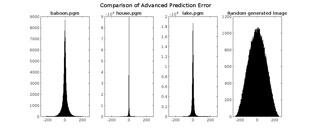
Comparison of Prediction Error with Different Algorithms

Discussion
Entropy Analysis
Real-world images (i.e. baboon, house and lake), as expected, have lower entropy compared to randomly generated images, indicating less randomness in their pixel values. This lower entropy suggests that real-world images may be more predictable and thus more favorable to compression.
Furthermore, within the category of real-world images, it’s worth noting that “house” demonstrates lower entropy than both “baboon” and “lake,” which exhibit similar levels of entropy. This discrepancy can be attributed to the tendency for “house” to display lower pixel variance compared to the other two images.
Zip Compression Analysis
Encoding rates achieved using “zip” compression are lower than entropy because dictionary encoding leverages the repetition of strings and symbols. Therefore, the theoretical limit is the entropy of symbol blocks, which in a signal exhibiting statistical dependencies, is lower than the entropy of individual symbols (once normalized for the block size).
In a signal lacking statistical dependencies, such as a randomly generated image, the entropy of symbol blocks closely resembles the entropy of the image itself. In fact, compression becomes disadvantageous compared to uncompressed images since it necessitates consideration of the space occupied by the dictionary and other data.
Among real-world images, as expected, we observe that “house” boasts significantly better compression due to its numerous repeated symbol strings, particularly evident in the sky and houses.
When comparing “baboon” and “lake,” despite “baboon” having lower entropy than “lake,” compression via zip yields better results for “lake.” This is attributed to “lake” exhibiting color groupings that repeat more frequently, for exemple the sky, despite having more color variance.
Simple Spatial Prediction Error Entropy
Let’s now experiment with simple spatial prediction. For each pixel, we’ll use the previous value as the predictor, except for the first pixel where we’ll use 128 as the prediction.
Once again, we observe that compressing the randomly generated image proves disadvantageous (compression ratio of about 0.92) because predicting a pixel from the previous one is impossible since the pixels are independent of each other.
Furthermore, we notice that compression improves as the colors of the image exhibit linear dependencies (without scattered and disjointed colors), thus achieving good prediction for “house” and fair prediction for “lake.” However, due to the high entropy of the baboon’s cheeks, compression of this particular image isn’t very effective, though still better than nothing.
Exp Golomb applied to Simple Spatial Prediction Error
When encoding the spatial prediction error obtained using our linear prediction algorithm with an Exp Golomb algorithm, we encounter values that are considerably penalized compared to the entropy value of our prediction algorithm. This entropy value could be approximated (with excellent accuracy) using an arithmetic encoder. However, the advantage of using an Exp Golomb algorithm over an arithmetic encoder lies in its much simpler implementation.
Nevertheless, this encoder significantly penalizes the compression of images where prediction errors are less concentrated around zero, i.e. with a higher signal sparsity. Specifically, randomly generated images and baboons are the two images most affected, even resulting in a disadvantage compared to uncompressed images. This is because their errors are more scattered, as easily seen from the histogram.
On the other hand, “house,” with its narrow histogram, receives a much lower penalty, thus giving results that are more than acceptable and even better than zip compression.
Advanced Spatial Prediction Error Entropy
Using an advanced spatial prediction instead in which the color of a pixel is estimated considering various factors:
- if the pixel is the first in the first row, 128 is used
- if it’s on the first row, the pixel to its left is used
- if it’s on the first column, the pixel above it is used
- If we’re on the last column, the prediction is based on the median value between the pixel above, the one to the left, and the one above and to the left
- In all the other cases, the pixel is predicted by calculating the median value between the pixel above, the one to the left, and the one above and to the right.

Using this prediction, we notice that compressing randomly generated images is disadvantageous, but a little less than using linear prediction. Because the median of three randomly generated numbers from 0 to k is closer to half of k, predicting a randomly generated number from 0 to k from this value is more advantageous than from a random number from 0 to k.
With this prediction, compression is better if the colors of the image are “patch-like.” We thus see an improvement in images like “lake” compared to all previously used compression systems. However, for images like “house” and “baboon,” the result is a little worse compared to linear prediction, as both photos are more linearly dependent than “patch-like.”
Exp Golomb applied to Advanced Spatial Prediction Error
When encoding the error obtained from advanced spatial prediction using an exp-Golomb algorithm, we observe a significant penalty compared to using an arithmetic encoder, as seen in the previous case with the use of exp-Golomb.
However, as mentioned earlier, this encoder heavily penalizes image compression when the error is not tightly clustered around zero. Consequently, it performs better than uncompressed images only in the cases of “house” and “lake,” where the error is more tightly clustered around zero. Moreover, it outperforms compression with linear prediction only in the case of “lake,” considering the highlighted details mentioned earlier.
Note
I’m not exactly an expert in image compression or anything like that, but due to my studies in computer engineering, I’ve found myself delving into various compression systems and conducting some comparisons. Thus, I’ve taken the opportunity to create this post.